6.4
The Black-Scholes Option Pricing Model
|
|
ere we use the
riskless hedge approach to determine option prices.
The formal details of this approach are provided in Appendix D, topic
D.4, Derivation
of the Black-Scholes Partial Differential Equation (PDE).
In
the riskless hedge approach, you may recall from the binomial model that we have
to construct a portfolio that is risk-free in every period.
Here, "every period" means continuously, since time evolves
continuously.
We
will show you here the option pricing solution, and then compare it to the
option pricing model obtained in a world of certainty.
This comparison provides some interesting insight into the nature of the
pricing model.
The
Black-Scholes Analysis
Black
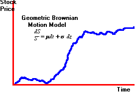
and Scholes assume a model for stock price dynamics that is formally described
as geometric Brownian motion and has the form:

Graphically,
this describes a process that wanders around as depicted in Figure 6.5.
Figure 6.5
Stock Price as a Function of Time

In
their seminal contribution to the theory of option pricing, Black and Scholes
solve the option pricing problem for an option defined on a stock whose price
follows such a process. They assume
that observed stock price movements resemble the behavior described by the
Brownian motion in Figure 6.5. From
this assumption they derive the implied price process for a European option
defined on the stock.
Since
both the stock and the option prices share a common source of uncertainty, this
derivation permits a riskless hedged portfolio to be constructed from the stock
and its underlying option. That is,
this portfolio eliminates the common source of uncertainty for "an
instant." As a result, this
portfolio in the absence of an arbitrage opportunity, will earn the
instantaneous risk-free rate.
By
creating this (instantaneously) riskless portfolio, Black and Scholes now have a
portfolio that contains an observed stock price, plus an unobserved option price
that equals a known risk-free rate. By
equating the instantaneous return from this hedged portfolio to the
instantaneous risk-free rate, Black and Scholes are able to derive and solve an
equation (often referred to as the Black-Scholes partial differential equation)
for the price of a European option.
This
price is important because a trader in a perfect market can rebalance the hedged
portfolio continuously over the remaining life of the option.
That is, the riskless hedged portfolio is maintained over time, and in
the absence of an arbitrage this portfolio will earn the continuously compounded risk-free rate. Therefore, the price
obtained by Black and Scholes from this riskless hedged portfolio is the
arbitrage free value of a European call option.
It should be noted that r in
this model refers to the continuously compounded risk free rate of interest. This is the rate of interest earned by the synthetic riskless
hedge that is maintained over the life of the option.
The
Black-Scholes Option Pricing Model
The
call option price is:

where

and
N( ) is the cumulative standard normal distribution.
Thus, N(d1)
is the probability that a normally distributed variable with mean 0 and variance
1 is less than d1.
Given
the value of a European call option, the price of a put option follows from the put call parity relationship (see Chapter 2, topic 2.9), that must
hold for European options in the absence of arbitrage.
Applying this relationship, the Black-Scholes price for a European put
option is:

Example
The current price of a stock is $50.
Consider a (European) call option with one year to maturity and with a
strike price of $50. The volatility is estimated at 25% per annum, and the
one-year continuously compounded interest rate is 10%.
What is the value of the call option?
Here,
S = 50
X = 50
s = 0.25
r = 0.1
T = 1
Using the Option Calculator, you can verify that the
call is worth $7.4879.
The value of a put option with the same parameters is
$2.7298.
It
is useful to compare the form of these pricing models with the option pricing
model under certainty.
Comparison
with Certainty Analysis
In
the certainty model, for a call option we obtained

and
the Black-Scholes price is

An
important implication of this valuation model is that the value of the option is
independent of the expected return from the underlying stock.
Equivalently, it is possible to value the option without knowing the true
probability distribution of the stock.
We can now return to the IBM options discussed earlier in the
certainty model. Recall that the
stock price less the present value of the dividend is $44.26, and the risk-free
interest rate is 2.867%. The
options information was
|
November
Options |
| ||
|
Call |
| ||
|
Strike |
Bid |
Ask |
|
|
35
|
9 3/8 |
9
7/8 |
|
|
40
|
4 7/8 |
5
|
|
|
45
|
1 1/16 |
1
3/8 |
|
|
50
|
1/4 |
3/8 |
|
The date of the information was Oct 15 1993, and the maturity
date of the options was November 20, 1993.
To value these options using the Black-Scholes formula, we
have
S = 44.26
r
= .02867
T =
0.0986
The value of T is
calculated by tallying the number of days to maturity and dividing
by 365.
The strike price, X,
ranges from 35 to 50. In
order to use the Black-Scholes formula, we need an estimate of
volatility. The
historical volatility of the return of IBM had traditionally been
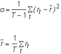
estimated at 30% (i.e., s = 0.3). This
is calculated as follows. Let
rt
= return from IBM stock between period t
-1 and t:

Then, s
is the standard deviation of the historical returns:

Typically, the standard deviation of returns is calculated on
a monthly or weekly basis; this return is then annualized to get a
number such as 30%.
For the options at hand, we calculated the values of the
options using three estimates of s :
30%, 35%, and 40%. This
leads to the following Black-Scholes prices for the call options,
as compared to the actual bids and asks in the market on October
15, 1993.
|
|
|
|
Volatility |
| ||
|
Strike |
Bid |
Ask |
0.3 |
0.35 |
0.4 |
|
|
|
|
|
|
|
|
|
|
35 |
9.375 |
9.875 |
9.37 |
9.38 |
9.42 |
|
|
40 |
4.875 |
5.000
|
4.64 |
4.79 |
4.98 |
|
|
45 |
1.437 |
1.875 |
1.39 |
1.66 |
1.94 |
|
|
50 |
0.25 |
0.375 |
0.28 |
0.36 |
0.54 |
|
For
convenience, we have converted the quoted bids and
asks into decimals.
As you can see, if s = 0.35, then
the Black-Scholes model yields prices within the
bid-ask spread, while option values obtained from
the historical figure are slightly lower than the
market prices.
Risk-Neutral Valuation Revisited
When
we can construct the riskless hedge, and arbitrage
arguments alone are sufficient to value derivative
securities, we once again obtain the risk-neutral
valuation principle (see Chapter 2, topic 2.7).
Since risk attitudes do not matter, the option has
the same value as in a hypothetical world where all
investors are risk-neutral.
In
this risk-neutral world, the value of the option is
the expected future value discounted by the continuously
compounded risk-free rate.
Before taking the expectation and discounting
it, note that the stock price must also equal
the expected future value discounted by the
risk-free interest rate.
But if the real world has risk-averse
investors, this cannot be the case. You can see the
problem as follows.
Let r be the risk-free
interest rate, and suppose that the risk adjusted
discount rate in the real world is r:
S = E(ST)e-rT
The
stock price in the real world is the future expected
value discounted by r.
If investors are risk-averse, then we expect r>r
(the difference between
r
and r
is called the risk premium).
In
a risk-neutral economy, we discount E(ST) by r, and this
value cannot possibly
equal S
since r > r.
The
problem is that the expected cash flows are too high
to be discounted by r.
To get the same stock price in the
risk-neutral world, we must reduce the expected
future cash flows.
This is done by changing the probability
distribution from the true distribution to what is
called the risk-neutral probability distribution.
You came across these probabilities in
Chapter 2, topic
2.7, Risk-Neutral
Valuation Principle.
Once
we have the risk-neutral probability distribution,
we can think of our two worlds moving through time
in a parallel fashion.
The first world is the real world.
The second world is the risk-neutral world,
where the distribution of stock prices has been
altered so as to be consistent with risk-neutrality.
We know the price of the option in the risk-neutral
world. It
is the expected future value discounted by the
risk-free rate; the expectation is taken with the
risk-neutral probability distribution. Risk-neutral valuation tells us that this is also the price
of the option in the real world.
The
trick is to identify these "risk-neutral
probabilities."
The Black-Scholes pricing model, however,
yields these probabilities in the form of N(d1) and N(d2).
As a result, the value of the call option
equals the stock price weighted by the risk-neutral
probability minus the present value of the strike
price weighted by another risk-neutral probability. This interpretation of N(d1)
and N(d2) as risk-neutral
probabilities is provided in Chapter 5, topic 5.2, Binomial Option Pricing: N-Periods, because the Black-Scholes
solution is exactly what we obtained in Appendix
C Chapter
5 Technical Topic:
Limiting Results.
In
the next topic Interpretation
of the Black-Scholes Mode,
we summarize some of the important implications of
the Black-Scholes model and the methodology used to
determine option prices.
In Chapter 13, topic 13.2, Applications:
Stock Options, you will be introduced to using
the online calculator
to determine the prices of commonly traded
stock options.
You may want to immediately apply the option
pricing model (using the calculator) to the stock
data provided.
 office (412)
9679367