In this topic, we describe some technical results that look at what happens to the binomial model when the number of periods goes to infinity.  You will see how the binomial model converges with the Black-Scholes model of option pricing.

Suppose that the option expires at time t, and n is some large number of periods into which we divide the time interval between now (which is time zero) and t.  We are interested in what happens when n goes to infinity.  If you think of the binomial tree, then this corresponds to being able to trade continuously (rather than at a discrete number of periods).

Once n is fixed, we need to rescale r, u, and d to account for the fact that a period can now be a very small interval of time.  For example, while u  =  1.5 may be appropriate over some extended period, it is clearly inappropriate if a period represents say, five seconds.

The adjustment to r, the 1 plus risk-free interest rate, is the simplest.  We want r raised to the power of t to be the value of one dollar at time t, so we define

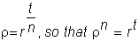
r is the 1 plus interest rate over a time interval of length n.

What about the adjustments to u and d?

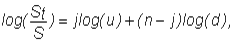
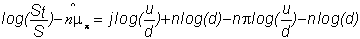
These can be motivated as follows.  Let ST be the (random) stock price in period t.  The expected, continuously compounded return from the stock between time t and t+1 is E{log(St+1/St).

A common assumption is that this return is independently and identically distributed,  with mean  m and variance  s2.  This means that over n periods, the expected return is  nm and the variance is  ns2.

Suppose that in n steps, we have j upticks and (n - j) downticks.  Then, we would have:

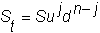
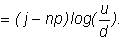
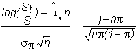
so that by dividing both sides by S and taking the log for the continuously compounded return:

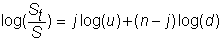
This can be rewritten as

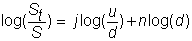
Taking expectations of both sides with respect to the binomial random variable j (the number of realized upticks), we get:

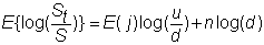
If q is the true probability of an uptick (which may be different from the risk-neutral probability p), then E(j) = nq.  The true probability determines the true expected return from the stock.  The variance of the return is

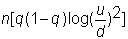
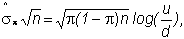
If, in the limit,  the binomial model is to yield that the expected return over t periods is mt and the variance of the return is st, we must choose u, d, and q so that

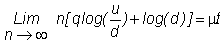
These conditions are met if

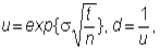
and

Previously, the value of a call option was determined to be:

where

(risk-neutral terminal value-weighted probability), and

(risk-neutral probability).

To determine the value of the call when n approaches infinity, we need to examine the limiting behavior of both

 .

The only other term that involves n is  r-n, which we know converges to r -t.

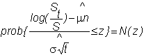
We will sketch an argument that shows that by substituting the values u and d, and taking the limit as n approaches infinity, the value of the call option converges to the Black-Scholes formula.  This formula is:

where

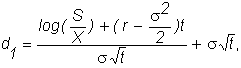
and

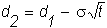
and N( ) is the cumulative normal distribution function.

There are two essential parts to the argument that characterizes the limiting behavior.

1)  Use the central limit theorem to derive the limiting distribution for the stock price.

2)  Parameterize the F's in terms of the stock price distribution to obtain the limits of the    probabilities.

The Distribution of St

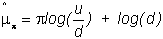
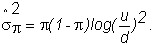
Let

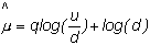
and

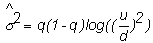
where  mt and  st are the mean and variance, respectively, of the continuously compounded stock return over the time interval [0,t].

The central limit theorem then implies that

where N(z) is the cumulative standard normal distribution.  This requires a technical regularity condition, which is satisfied.  Thus, in the limit, log(St/S) is normally distributed with mean  mt and variance  s2t.

Note that we already knew that the mean and variance of this return were mt and  s2t; what the theorem gives us is that the return is normally distributed.  It implies that St is lognormally distributed with mean (m + s2/2)t and variance  s2t.

The Binomial Probabilities

In this section, we will go through a similar construction using the risk-neutral probability,  p, instead of the true probability, q.

Let

and

If we have j upticks in n moves then

so

Also

so

F(m,n;p) is the probability that a binomial random variable, which takes on the value 1 with probability  p and 0 with probability (1-p), leads to at least m draws of 1 in n attempts.  Therefore, 1 -  F(m,n;p) is the probability of less than m draws of 1 in n attempts.  If j is the number of draws of 1, or equivalently the sum of the n draws, then j has a binomial distribution with mean np and variance np(1 - p).  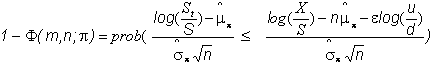Thus,

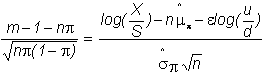
 From the equation immediately preceding this, we then get

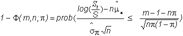
Recall that m is the smallest integer such that Sumdn-m  >  X, so that we can write

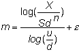
for some  e between 0 and 1.

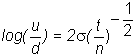
Substituting for m, and using the relations

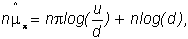
and

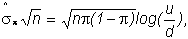
it is easy to verify that

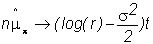
Therefore,

The limiting behavior then depends on the behavior of

and

It is easy to see that

goes to zero, since

The final step in the argument is to show that

and

This can be done by examining the limit of  p as n gets large.  Recalling the definition of p, both the numerator and denominator go to zero.  The limiting behavior is then determined by application of L'Hopital's rule.  We do not go through these steps here.

The result, then, is that

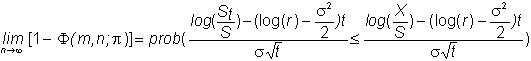
so that

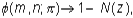
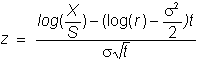
where

Symmetry of the normal distribution implies 1 - N(z) = N(-z), so we can write

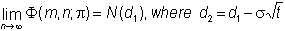
Finally, we obtain the value of the call in the limit:

This is the Black-Scholes formula.

In the next chapter, The Black-Scholes Option Pricing Model, the continuous time approach is presented to derive the option pricing model.