n this topic, we apply the risk-neutral valuation technique to value a European call option that lasts for n-periods.  The presentation is based upon the work of Cox, Ross, and Rubinstein (1979). 

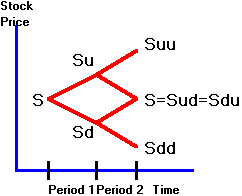
The tree for the stock in the two-period problem is shown in Figure 5.1.

Figure 5.1

Binomial Tree:  2-Period

In this case, we can write the call option value with respect to risk-neutral probabilities  p as:

This two-period form can be rearranged into the general N-period binomial option pricing model by summing over the 2n possible paths that the underlying stock price can take.

To take a closer look at the derivation of how the N-period model generalizes the two-period model, you can read topic 5.3, Binomial Option Pricing Model:  N-Period Derivation.

The n-period binomial option pricing model is expressed as:

Here, p is the risk-neutral probability of a realized uptick u, and q = pu/r, which has the property that 0 < q < 1 because  q = u(r - d)/(r(u - d)) and u > r.  We can interpret  q  as a "risk-neutral terminal value-weighted probability." F is the probability of at least m upticks occurring from n ticks computed relative to risk-neutral probabilities p, and risk-neutral value-weighted probabilities q.

This model includes two binomial probability distribution terms as a function of n, the number of periods, and m, which is the smallest number of upticks required for the call option to finish "in-the-money."

The first term is the present value of the expected revenue from exercising an in-the-money option.  This term is not simply equal to S times the probability of the call being in-the-money, because the expected revenue depends on the terminal stock price associated with each path.  The critical information associated with a path and its terminal value is the number of upticks realized plus the constants u and r along the path.  Therefore, we can calculate the expected revenue from the current stock price weighted by the risk-neutral terminal value-weighted probability.

The second term is the (risk-neutral) probability that the call option will be in-the-money multiplied by the exercise price and discounted by the risk-free rate.  Therefore, it is the present value of the expected exercise cost.

If you want to see the derivation of how the N-period model generalizes the two-period model, see  topic 5.3, Binomial Option Pricing Model:  N-Period Derivation, otherwise you can skip to the limiting behavior of the binomial option pricing model, as periods become smaller and smaller, in  topic 5.4, Binomial Option Pricing:  Limiting Results).