3.2
Two-Period Binomial Model: European
Option
|
T |
he
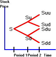
general two-period binomial model is depicted in Figure 3.1:
Figure 3.1
Two-Period Binomial Tree

The
notation we use to develop the general two-period binomial model for European
options is:
S
= current stock price;
C
= price of the call option;
X = strike
price;
P = price of
the put option;
u = uptick in
either period;
d = downtick
in either period; and
r = 1 plus
the (per period) risk-free interest rate
The
options will mature at the end of period 2.
Suppose
that at the end of period 1, the stock price moves either up to Su
or down to Sd where:
Su = high
stock price at the end of period 1 (state H);
Sd = low
stock price at the end of period 1 (state L).
In
period 2, there are four possible stock values.
Let
Suu = high
stock price at the end of period 2, if the stock price is high in period 1;
Sud = low
stock price at the end of period 2, if the stock price is high in period 1;
Sdu = high
stock price at the end of period 2, if the stock price is low in period 1;
Sdd = low
stock price at the end of period 2, if the stock price is low in period 1.
If
you are working on the computer, Figure 3.1 is available as a popup window by
clicking on Two-Period Tree. This
popup also contains the one-period option pricing model.
You may find it useful to have this popup open while working through this
topic.
We
start by valuing the call option. The
call is valued recursively by working backwards through the tree.
We start at the end; you know that the value of the call option at the
end is one of
Cuu = max { 0, Suu - X
}
Cud
= max { 0, Sud - X }
Cdu
= max { 0, Sdu - X }
Cdd = max { 0, Sdd - X
}
(We
assume that Suu > X ; otherwise the option never has any value.)
Now,
move back one period. Suppose we
are at Su (i.e., the first tick was an uptick). At this point, we have only one period left, so we know from
Chapter 2 how to calculate Cu.
Similarly, we know how to calculate Cd.
Now, come back to the beginning, where we want to calculate C.
Here, we simply have a one-period binomial model again, where the call
value on the uptick is Cu
and that on a downtick is Cd.
We
will repeat these steps in detail below. The
key step is simply that by working backward, we reduce the two-period problem to
a sequence of one-period problems. At
each point, we apply the one-period model (see topic 2.4, Call
Option Valuation: A Riskless Hedge Approach developed in Chapter 2).
The
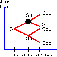
detailed calculations are as follows. Let Cu be the value of the call option at the node shown by a black
circle on the tree in Figure 3.2 and let ku be the hedge ratio.
At this node, we had an uptick in the first period.
Figure 3.2
Position in Tree After an Uptick

In
the one-period problem we solved for the value of the call option at the
beginning of period 1, C, as:

All
we have to do to this is substitute Su
for S, Suu
for Su and so on, resulting in:

where

Similarly,
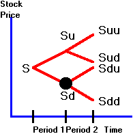
you can calculate the value of the call option at the realized downtick node
marked in black in Figure 3.3.
Figure 3.3
Position in Tree After a Downtick

By
applying the one-period model to this node, we get:

where

Finally,
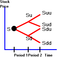
we come to the first node, the black circle in Figure 3.4.
Figure 3.4
The First Node

Here,
we can directly apply the formula from the one-period model:

where

You
can see that there is only one difference between how we approached the
two-period problem and how we approached the one-period problem.
In the one-period problem, we calculated Cu
and Cd from the terminal
value of the option contract (i.e., the max conditions).
In the two-period problem, we could use this information only at the end
of period 2. As a result, we first
had to calculate Cu and Cd
from the period 2 terminal value information using the one-period option pricing
model. We could then use these
values for Cu and Cd
(in place of the terminal values used in the one-period model) and then repeat
the application of the one-period model.
You
may want to calculate the general form of the European put option pricing model
as an exercise. Or, you can derive
this simply by applying the Put-Call Parity
Relationship (See Chapter 2, topic 2.9), at each node.
That is, if you know the value of a European option and the stock price
at each node, then the value of the European put option is:

The two-period model is easy to
extend to any number of periods.
It can also be used to handle very complex option pricing problems.
For example, it is not necessary that
u and d
be constant over time, or that the risk-free interest rate be constant (as long
as it is deterministic). A formal
treatment of the multi-period binomial analysis is provided in Chapter 5,
the N-Period Binomial Option Pricing
Model.
Next,
we introduce options that you can exercise at any time before maturity.
Such options are called American options. You can work
through the American option problem in the next topic, American
Call Option: Zero-Dividend Case.
 office (412)
967-9367